Linear Inference Sessions

An overview and example of a linear inference model for performing tasks such as GWAS in HFL

The built-in model package iai_linear_inference trains a bundle of linear models for the target of interest against a specified list of predictors. It obtains the coefficients and variance estimates, and also calculates the p-values from the corresponding hypothesis tests. Linear inference is particularly useful for genome-wide association studies (GWAS), to identify genomic variants that are statistically associated with a risk for a disease or a particular trait.

This is a horizontal federated learning (HFL) model package.

The integrateai_linear_inference.ipynb, located in the sample-notebook folder of the SDK package, demonstrates this model package using the sample data that is available for download from the integrate.ai web dashboard.

Follow the instructions in the Environment Setup section to prepare a local test environment for this tutorial.

Overview of the iai_linear_inference package

There are two strategies available in the package:

1. LogitRegInference - for use when the target of interest is binary

2. LinearRegInference - for use when the target is continuous

Example model_config for a binary target:

model_config_logit = {
    "strategy": {"name": "LogitRegInference", "params": {}},
    "seed": 23,  # for reproducibility
}

The data_config dictionary should include the following three fields.

• target: the target column of interest

• shared_predictors: predictor columns that should be included in all linear models. For example, the confounding factors like age, gender in GWAS.

• chunked_predictors: predictor columns that should be included in the linear model one at a time. For example, the gene expressions in GWAS.

The columns in all the fields can be specified as either names/strings or indices/integers.

Example data_config:

data_config_logit = {
    "target": "y",
    "shared_predictors": ["x1", "x2"],
    "chunked_predictors": ["x0", "x3", "x10", "x11"]
}

With this example data configuration, the session trains four logistic regression models with y as the target, and x1, x2 plus any one of x0, x3, x10, x11 as predictors.

Create a training session

For this example, there are two (2) training clients and the model is trained over five (5) rounds.

training_session_logit = client.create_fl_session(
    name="Testing linear inference session",
    description="I am testing linear inference session creation through a notebook",
    min_num_clients=2,
    num_rounds=5,
    package_name="iai_linear_inference",
    model_config=model_config_logit,
    data_config=data_config_logit,
).start()

training_session_logit.id

Argument (type)	Description
name (str)	Name to set for the session
description (str)	Description to set for the session
min_num_clients (int)	Number of clients required to connect before the session can begin
num_rounds (int)	Number of rounds of federated model training to perform
package_name(str)	Name of the model package to be used in the session
model_config (Dict)	Contains the model configuration to be used for the session
data_config (Dict)	Contains the data configuration to be used for the session

Ensure that you have downloaded the sample data. If you saved it to a location other than your Downloads folder, specify the data_path to the correct location.

data_path = "~/Downloads/synthetic"

Start the training session

This example demonstrates starting a training session locally. The clients joining the session are named client-1-inference and client-2-inference, respectively.

import subprocess

client_1 = subprocess.Popen(
    f"iai client train --token {IAI_TOKEN} --session {training_session_logit.id} --train-path {data_path}/train_silo0.parquet --test-path {data_path}/test.parquet --batch-size 1024 --client-name client-1-inference --remove-after-complete",
    shell=True,
    stdout=subprocess.PIPE,
    stderr=subprocess.PIPE,
)

client_2 = subprocess.Popen(
    f"iai client train --token {IAI_TOKEN} --session {training_session_logit.id} --train-path {data_path}/train_silo1.parquet --test-path {data_path}/test.parquet --batch-size 1024 --client-name client-2-inference --remove-after-complete",
    shell=True,
    stdout=subprocess.PIPE,
    stderr=subprocess.PIPE,
)

Poll for session status

Use a polling function, such as the example below, to wait for the session to complete.

import time

current_round = None
current_status = None
while client_1.poll() is None or client_2.poll() is None:
    output1 = client_1.stdout.readline().decode("utf-8").strip()
    output2 = client_2.stdout.readline().decode("utf-8").strip()
    if output1:
        print("silo1: ", output1)
    if output2:
        print("silo2: ", output2)

    # poll for status and round
    if current_status != training_session_logit.status:
        print("Session status: ", training_session_logit.status)
        current_status = training_session_logit.status
    if current_round != training_session_logit.round and training_session_logit.round > 0:
        print("Session round: ", training_session_logit.round)
        current_round = training_session_logit.round
    time.sleep(1)

output1, error1 = client_1.communicate()
output2, error2 = client_2.communicate()

print(
    "client_1 finished with return code: %d\noutput: %s\n  %s"
    % (client_1.returncode, output1.decode("utf-8"), error1.decode("utf-8"))
)
print(
    "client_2 finished with return code: %d\noutput: %s\n  %s"
    % (client_2.returncode, output2.decode("utf-8"), error2.decode("utf-8"))
)

View training metrics and model details

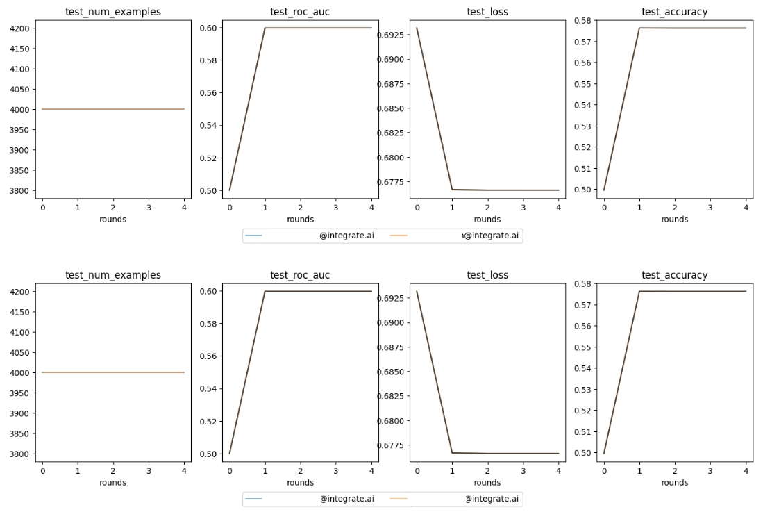
Once the session is complete, you can view the training metrics and model details such as the model coefficients and p-values. In this example, since there are a bundle of models being trained, the metrics are the average values of all the models.

training_session_logit.metrics().as_dict()

Example output:

{'session_id': '3cdf4be992',
 'federated_metrics': [{'loss': 0.6931747794151306},
  {'loss': 0.6766608953475952},
  {'loss': 0.6766080856323242},
  {'loss': 0.6766077876091003},
  {'loss': 0.6766077876091003}],
 'client_metrics': [{'[e-mail]:dedbb7e9be2046e3a49b28b0131c4b97': {'test_loss': 0.6931748060977674,
    'test_accuracy': 0.4995,
    'test_roc_auc': 0.5,
    'test_num_examples': 4000},
   '[e-mail]:339d50e453f244ed9cb2662ab2d3bb66': {'test_loss': 0.6931748060977674,
    'test_accuracy': 0.4995,
    'test_roc_auc': 0.5,
    'test_num_examples': 4000}},
  {'[e-mail]:dedbb7e9be2046e3a49b28b0131c4b97': {'test_num_examples': 4000,
    'test_loss': 0.6766608866775886,
    'test_roc_auc': 0.5996664746664747,
    'test_accuracy': 0.57625},
   '[e-mail]:339d50e453f244ed9cb2662ab2d3bb66': {'test_num_examples': 4000,
    'test_loss': 0.6766608866775886,
    'test_accuracy': 0.57625,
    'test_roc_auc': 0.5996664746664747}},
  {'[e-mail]:339d50e453f244ed9cb2662ab2d3bb66': {'test_loss': 0.6766080602706078,
    'test_accuracy': 0.5761875,
    'test_num_examples': 4000,
...
   '[e-mail]:339d50e453f244ed9cb2662ab2d3bb66': {'test_accuracy': 0.5761875,
    'test_roc_auc': 0.5996632246632246,
    'test_num_examples': 4000,
    'test_loss': 0.6766078165060236}}],
 'latest_global_model_federated_loss': 0.6766077876091003}

Plot the metrics

training_session_logit.metrics().plot()

Example output:

Retrieve the trained model

The LinearInferenceModel object can be retrieved using the model's as_pytorch method. And the relevant information such as p-values can be accessed directly from the model object.

model_logit = training_session_logit.model().as_pytorch()

Retrieve the p-values

pv = model_logit.p_values()
pv

The .p_values() function returns the p-values of the chunked predictors.

Example output:

x0      112.350396
x3      82.436540
x10     0.999893
x11     27.525280
dtype: float64

Summary information

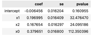
The .summary method fetches the coefficient, standard error, and p-value of the model corresponding to the specified predictor.

summary_x0 = model_logit.summary("x0")
summary_x0

Example output:

Making predictions

You can also make predictions with the resulting bundle of models when the data is loaded by the ChunkedTabularDataset from the iai_linear_inference package. The predictions will be of shape (n_samples, n_chunked_predictors) where each column corresponds to one model from the bundle.

from torch.utils.data import DataLoader
from integrate_ai_sdk.packages.LinearInference.dataset import ChunkedTabularDataset

ds = ChunkedTabularDataset(path=f"{data_path}/test.parquet", **data_config_logit)
dl = DataLoader(ds, batch_size=len(ds), shuffle=False)
x, _ = next(iter(dl))
y_pred = model_logit(x)
y_pred

Example output:

tensor([[0.3801, 0.3548, 0.4598, 0.4809],
        [0.4787, 0.3761, 0.4392, 0.3579],
        [0.5151, 0.3497, 0.4837, 0.5054],
        ...,
        [0.7062, 0.6533, 0.6516, 0.6717],
        [0.3114, 0.3322, 0.4257, 0.4461],
        [0.4358, 0.4912, 0.4897, 0.5110]], dtype=torch.float64)