HFL Gradient Boosted Models (HFL-GBM)

An overview of the integrate.ai implementation of GBM for HFL

Gradient boosting is a machine learning algorithm for building predictive models that helps minimize the bias error of the model. The gradient boosting model provided by integrate.ai is an HFL model that uses the sklearn implementation of HistGradientBoostingClassifier for classifier tasks and HistGradientBoostingRegresssor for regression tasks.

The GBM sample notebook (integrateai_api_gbm.ipynb) provides sample code for running the SDK, and should be used in parallel with this tutorial. This documentation provides supplementary and conceptual information to expand on the code demonstration.

Prerequisites

1. Complete the Environment Setupfor your local machine.

2. Open the integrateai_api_gbm.ipynb notebook to test the code as you walk through this tutorial.

Review the sample Model Configuration

integrate.ai has a model class available for Gradient Boosted Models, called iai_gbm. This model is defined using a JSON configuration file during session creation.

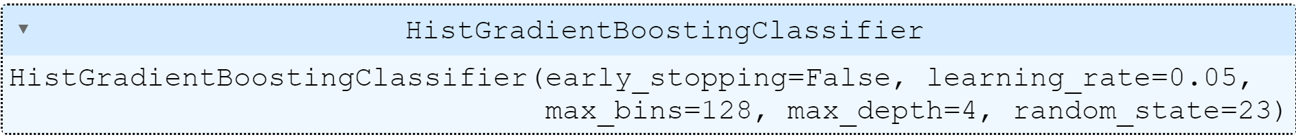
1. The strategy for GBM is HistGradientBoosting.

2. You can adjust the following parameters as needed:

   1. max_depth - Used to control the size of the trees.

   2. learning_rate - (shrinkage) Used as a multiplicative factor for the leaves values. Set this to one (1) for no shrinkage.

   3. max_bins - The number of bins used to bin the data. Using less bins acts as a form of regularization. It is generally recommended to use as many bins as possible.

   4. sketch_relative_accuracy - Determines the precision of the sketch technique used to approximate global feature distributions, which are used to find the best split for tree nodes.

3. Set the machine learning task type to either classification or regression.

   1. Specify any parameters associated with the task type in the params section.

4. The save_best_model option allows you to set the metric and mode for model saving. By default this is set to None, which saves the model from the previous round, and min.

Example model configuration JSON:

model_config = {
    "strategy": {
        "name": "HistGradientBoosting",
        "params": {}
    },
    "model": {
        "params": {
            "max_depth": 4, 
            "learning_rate": 0.05,
            "random_state": 23, 
            "max_bins": 128,
            "sketch_relative_accuracy": 0.001,
        }
    },

    "ml_task": {"type": "classification", "params": {}}, 
    
    "save_best_model": {
        "metric": None,
        "mode": "min"
    },
  }

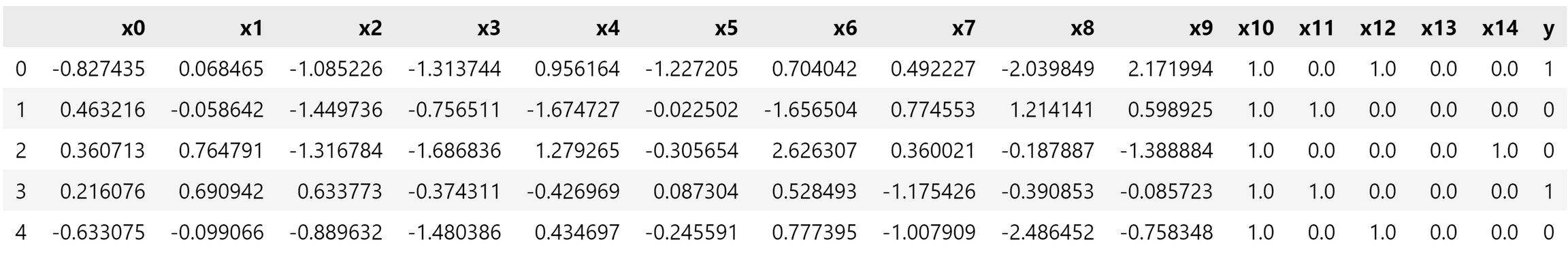
The notebook also provides a sample data schema. For the purposes of testing GBM, use the sample schema, as shown below.

data_schema = {
    "predictors": ["x0", "x1", "x2", "x3", "x4", "x5", "x6", "x7", "x8", "x9", "x10", "x11", "x12", "x13", "x14"],
    "target": "y",
}

For more about data schemas, see Create a Custom Data Loader.

Create and run a GBM training session

Federated learning models created in integrate.ai are trained through sessions. You define the parameters required to train a federated model, including data and model configurations, in a session.

Create a session each time you want to train a new model.

The following code sample demonstrates creating and starting a session with two training clients (two datasets) and ten rounds (or trees). It returns a session ID that you can use to track and reference your session.

training_session = client.create_fl_session(
    name="HFL session testing GBM",
    description="I am testing GBM session creation through a notebook",
    min_num_clients=2,
    num_rounds=10,
    package_name="iai_gbm",
    model_config=model_config,
    data_config=data_schema,
).start()

training_session.id

Argument (type)	Description
name (str)	Name to set for the session
description (str)	Description to set for the session
min_num_clients (int)	Number of clients required to connect before the session can begin
num_rounds (int)	Number of rounds of federated model training to perform. This is the number of trees to train.
package_name(str)	Name of the model package to be used in the session. For GBM sessions, use iai_gbm.
model_config (Dict)	Name of the model configuration to be used for the session
data_config (Dict)	Name of the data configuration to be used for the session

Start the training session

The next step is to join the session with the sample data. This example has data for two datasets simulating two clients, as specified with the min_num_clients argument. Therefore, to run this example, you will call subprocess.Popen twice to connect each dataset to the session as a separate client.

The session begins training once the minimum number of clients have joined the session.

Each client runs as a separate Docker container to simulate distributed data silos.

If you extracted the contents of the sample file to a different location than the default, change the data_path in the sample code before attempting to run it.

Example:

import subprocess

data_path = "~/Downloads/synthetic"

client_1 = subprocess.Popen(f"iai client train --token {IAI_TOKEN} --session {training_session.id} --train-path {data_path}/train_silo0.parquet --test-path {data_path}/test.parquet --batch-size 1024 --client-name client-1 --remove-after-complete",
    shell=True,
    stdout=subprocess.PIPE,
    stderr=subprocess.PIPE,
)

client_2 = subprocess.Popen(f"iai client train --token {IAI_TOKEN} --session {training_session.id} --train-path {data_path}/train_silo1.parquet --test-path {data_path}/test.parquet --batch-size 1024 --client-name client-2 --remove-after-complete",
    shell=True,
    stdout=subprocess.PIPE,
    stderr=subprocess.PIPE,
)

where

• data_path is the path to the sample data on your local machine

• IAI_TOKEN is your access token

• training_session.id is the ID returned by the previous step

• train-path is the path to and name of the sample dataset file

• test-path is the path to and name of the sample test file

• batch-size is the size of the batch of data

• client-name is the unique name for each client

Poll for Session Results

Sessions take some time to run. In the sample notebook and this tutorial, we poll the server to determine the session status.

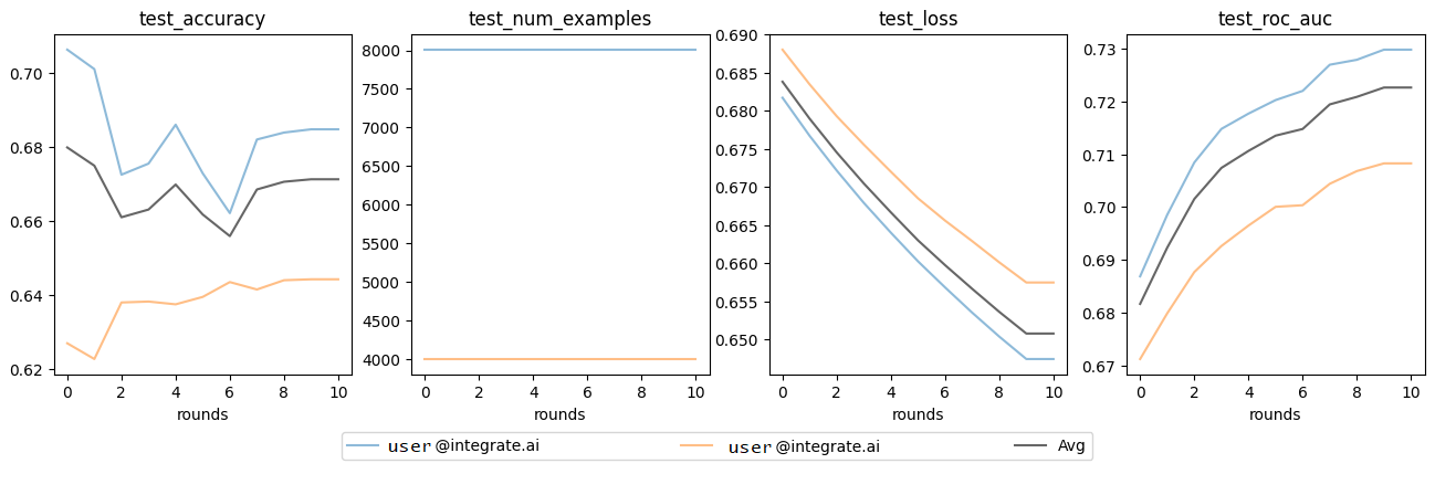
View the training metrics

After the session completes successfully, you can view the training metrics and start making predictions.

1. Retrieve the model metrics as_dict.

2. Plot the metrics.

// Retrieve the model metrics

training_session.metrics().as_dict()

Example output

Output exceeds the size limit. Open the full output data in a text editor
{'session_id': '9fb054bc24',
 'federated_metrics': [{'loss': 0.6876291940808297},
  {'loss': 0.6825978879332543},
  {'loss': 0.6780059585869312},
  {'loss': 0.6737175708711147},
  {'loss': 0.6697578155398369},
  {'loss': 0.6658972384035587},
  {'loss': 0.6623568458259106},
  {'loss': 0.6589517279565335},
  {'loss': 0.6556690569519996},
  {'loss': 0.6526266353726387},
  {'loss': 0.6526266353726387}],
 'rounds': [{'user info': {'test_loss': 0.6817054933875072,
    'test_roc_auc': 0.6868823702288674,
    'test_accuracy': 0.7061688311688312,
    'test_num_examples': 8008},
   'user info': {'test_accuracy': 0.5720720720720721,
    'test_num_examples': 7992,
    'test_roc_auc': 0.6637941733389123,
    'test_loss': 0.6935647668830733}},
  {'user info': {'test_accuracy': 0.5754504504504504,
    'test_roc_auc': 0.6740578481919338,
    'test_num_examples': 7992,
    'test_loss': 0.6884922753070576},
   'user info': {'test_loss': 0.6767152831608197,
...
   'user info': {'test_loss': 0.6578156923815811,
    'test_num_examples': 7992,
    'test_roc_auc': 0.7210704078520924,
    'test_accuracy': 0.6552802802802803}}],
 'latest_global_model_federated_loss': 0.6526266353726387}

// Plot the metrics

fig = training_session.metrics().plot()

Example plots:

Example plots from sample notebook and sample data

model = training_session.model().as_sklearn()
model

Example of the classifier model from the notebook

Load the test data

import pandas as pd

test_data = pd.read_parquet(f"{data_path}/test.parquet")
test_data.head()

Example of loading the test data from the sample notebook

Convert test data to tensors

Y = test_data["y"]

X = test_data[["x0", "x1", "x2", "x3", "x4", "x5", "x6", "x7", "x8", "x9", "x10", "x11", "x12", "x13", "x14"]]

Run model predictions

model.predict(X)

Result: array([0, 1, 0, ..., 0, 0, 1])

from sklearn.metrics import roc_auc_score
y_hat = model.predict_proba(X)
roc_auc_score(Y, y_hat[:, 1])

Result: 0.7082738332738332

When the training sample sizes are small, this model is more likely to overfit the training data.